The Aerospace Design Toolbox is now available on Matlab Central.  This release includes examples on how to use the various functions to integrate with XFoil, AVL, and more.

I’ve recently switched to using Github for my open source projects.  As apart of this transition, I’ve been restructuring some of my old code.  This has lead to the creation of the aerospace-design-toolbox (ADT).

This Matlab toolbox is built from the Mavl code base.  The biggest difference between the two is scope.  While Mavl was designed to address the full scope of the design process from modeling to analysis, the ADT simply supports loading data from other aerospace software into Matlab.  Currently the ADT reads output files from AVL and Xfoil.  It can additionally read prop data in the format used by the UIUC propeller database.  For more information on what is and isn’t supported please see the README.m file in the repository.

At this time the toolbox is just a set of utility functions.  In the near term development will focus on converting the code into a standard toolbox that will integrate better with Matlab.

The following details the mission performance of NC State University’s Aerial Robotics Club at the 10th annual AUVSI Student Unmanned Systems competition.

The autopilot successfully executed a fully autonomous take-off before switching over to manual control due to an error in the autopilot’s altitude configuration.  It was later determined to have been operator error caused by improper zeroing of the altitude.  Autonomous control was regained by flying at a higher altitude than originally planned.  The waypoints, search pattern, and emergent target pattern were flown at this fixed altitude.

One special feature added this year was a laser altimeter.  Despite early concerns of a failure, the altimeter performed well through out the mission.

The SRIC message was determined to be:

John Paul Jones, defeated British ship Serapis in the Battle of Flamborough Head on 23 September 1779

The targets this year spelled out the phrase, “Fear the goat”.  This apparently has something to do with the mascot of the United States Naval Academy “Bill the goat”.

The emergent target this year was a wounded hiker and his backpack.  Most of these details were visible in the images taken with the exception of his wounds.

Automatic code generation is a powerful tool that when combined with Simulink promises important benefits to students and highly complicated applications alike.  Mathworks distributes an Arduino Blockset for Simulink.  The Arduino platform is a desirable to use because of its simple architecture and available hardware.  These hardware options include the ArdupilotMega (APM) which includes sensors and pinouts that will make it easier to integrate into a future aerial vehicle.

While the 2012a version only requires the base Matlab and Simulink packages, NCSU does not currently provide the 2012a version to students.  Instead the 2011a version was used since it was available.  It is not expected that there will be problems using the work done with 2011a in the 2012a release.

The base Arduino blockset includes blocks for Analog and Digital I/O as well as serial communication.  To take full advantage of the capabilites of the APM, additional blocks for SPI, I2C, PPM, and Servos are needed.  Development of a servo blocks has been the focus of this last week.

  The new blocks, shown in blue, allow for the configuration and control of servos attached to the APM.  An interesting note  is that although the APM only has 8 servo lines broken out on the side, there are an additional 3 lines (PL3, PB5, and PE3) that can be configured to output PWM commands. These lines are broken out from the APM base-board, but are not available on the sensor-shield “Oilpan”.

With just the blocks from the base, shown in yellow, and the new servo blocks it is already possible to access quite a few of the APM’s functions.  The demonstration program shown above commands two servos through a sin wave motion.  Data is read from the serial port allowing for the functionality of Servo 1 to be switched between sin wave and center position.

The Piccolo Command Center (PCC) software allows an operator to plan and execute flights using the Piccolo autopilot.  However, it can be difficult to analyze post-flight telemetry.  Additionally, access to the PCC software is limited.

To address this problem I created a matlab function “log2kml.m” to convert Piccolo log files into KML files readable by Google Earth (GE).  This function reads the space delimited log file into Matlab.  It then filters out bad GPS points.  Finally it steps through the data to create a KML polyline.  The line is segmented based on the flight mode to clarify what the autopilot was doing.  The function uses the KML toolbox created by Rafael Fernandes de Oliveira.  It can be found at http://www.mathworks.com/matlabcentral/fileexchange/34694.  This toolbox is put together well and was easy to use.

The results shown below make the high performance of the autopilot clear.  Since the points are 3D there is some distortion of the actual ground path.

AUVSI 2011 NCSU Competition Run

This visualization  allows us to analyze certain maneuvers much more easily.  A point of concern on autonomous take-offs has been a “dip” that occurs as the aircraft switches from prioritizing altitude to prioritizing airspeed.  Using the “Elevation Profile” tool in GE alongside the flight path allows for a clear observation of the performance.

Autonomous Take-off Performance

It can now clearly be seen that the aircraft does level out, but does not lose altitude.  We can also determine that it levels off at an altitude of 21 meters or 68 feet above ground level.  This new knowledge can now be applied to improving future performance, or at least avoiding flying in to trees at the end of the runway.

For comparison a screenshot from the PCC is shown below.  Since the blue line representing the flight path is so course, the fine motion of the aircraft is only apparent when animated.  The profile view only shows the current position of the aircraft.  Finally, the 3D view isn’t apart of the base software package resulting in the “License Required” text being splashed across the screen.

PCC View

Mark Drela’s Athena Vortex Lattice (AVL)  program is a powerful tool for aerodynamic analysis.  Automating AVL runs using Matlab not only saves time, but eliminates human error when plugging through a large range of run cases.  In combination with tools for parsing the results and editing the models this automation may also enable design methods such as genetic algorithms and other iterative approaches.

Included below is a zip file containing the example script detailed here as well as a set of sample AVL files copied from the AVL source directory.  You will need to download AVL yourself and place the executable in the unzipped folder with the other files. Alternately, you may change the path to the avl executable in the last line of the script.  This tutorial was tested against avl 3.27.  Version 3.16 may have issues.

runAVL

Creating the run file

The run file to be created is simply a batch script that will be fed into AVL.  This will cause AVL to act as though the commands in the batch file are being typed in by a user.  The process begins by creating a blank file to put the batch script in.

%% Create run file %Open the file with write permission fid = fopen('.allegro.run', 'w');

Once this is complete, each line of the batch script is “printed” to the file by the fprintf command.  First, the aircraft’s avl and mass file are loaded into AVL.  The MSET command is executed to apply the mass parameters to all the run cases.  Then graphics are disabled to allow the program to run silently in the background.

%Load the AVL definition of the aircraft
fprintf(fid, 'LOAD %s\n', strcat(filename,'.avl'));

%Load mass parameters
fprintf(fid, 'MASS %s\n', strcat(filename,'.mass'));
fprintf(fid, 'MSET\n');
%Change this parameter to set which run cases to apply
fprintf(fid, '%i\n',   0); 

%Disable Graphics
fprintf(fid, 'PLOP\ng\n\n');

Once the setup is complete, the run case is defined and executed.  In this instance the C1 command is used to “set level or banked  horizontal flight constraints”.  The velocity is then set.  Depending on the purpose of the run case you may also use commands such as commented out under “Options for trimming”.  The case is then run using the X command.

%Open the OPER menu
fprintf(fid, '%s\n',   'OPER');   

%Define the run case
fprintf(fid, 'c1\n',   'c1');
fprintf(fid, 'v %6.4f\n',velocity);
fprintf(fid, '\n');

%Options for trimming %fprintf(fid, '%sn', 'd1 rm 0'); %Set surface 1 so rolling moment is 0 %fprintf(fid, '%sn', 'd2 pm 0'); %Set surface 2 so pitching moment is 0

%Run the Case
fprintf(fid, '%s\n',   'x');

Once the run is complete, the desired data in the OPER menu is saved to files for post analysis.  This example shows how to save the stability derivatives (ST) and body-axis derivatives (SB) data.  Other data that can be saved off in a similar fashion as shown below include:

• ST  stability derivatives
• SB  body-axis derivatives
• RE  reference quantities
• FT  total   forces
• FN  surface forces
• FS  strip   forces
• FE  element forces
• VM  strip shear,moment
• HM  hinge moments

%Save the st data
fprintf(fid, '%s\n',   'st');
fprintf(fid, '%s%s\n',basename,'.st');
%Save the sb data
fprintf(fid, '%s\n',   'sb');
fprintf(fid, '%s%s\n',basename,'.sb');

%Drop out of OPER menu
fprintf(fid, '%s\n',   '');

Other data may also be obtained by leaving the OPER menu and entering the MODE menu.  This eigenvalue data can be useful for analyzing an aircraft’s stability.

%Switch to MODE menu
fprintf(fid, '%s\n',   'MODE');
fprintf(fid, '%s\n',   'n');
%Save the eigenvalue data
fprintf(fid, '%s\n',   'w');
fprintf(fid, '%s%s\n', basename,'.eig');   %File to save to

%Exit MODE Menu
fprintf(fid, '\n');

Once all the desired runs have been computed and saved, it is important to use the return key character ‘n’ to return to the top level menu before issuing the Quit command to exit out of AVL and back to the command line. With the script complete the batch script file is closed.

%Quit Program
fprintf(fid, 'Quit\n'); 

%Close File
fclose(fid);

Executing the script

Files whose names conflict with new files to be generated should be moved out of the target directory or deleted before running the script.

[status,result] =dos(strcat('del ','allegro.st'));

Execution of the script from matlab is acheived by simply using the below command.  The dos command tells matlab to execute the string argument on the command line.  The instruction tells the OS feed the allegro.run file in the local directory to the avl executable at the absolute address shown.  The dos function also returns status and result data.  The status variable will get the final return state of the execution, nominally a 0 unless the program crashed.  The result variable will contain all the text that would have been printed to the screen if executed from the command line.

[status,result] = dos('C:avl.exe < .allegro.run');

With this complete the batch script will have successfully executed your run case or will have crashed.  To debug your batch script it is helpful to look through the result variable’s data.  Also helpful is to manually type in a script so that you can see more easily what the program is trying to do.

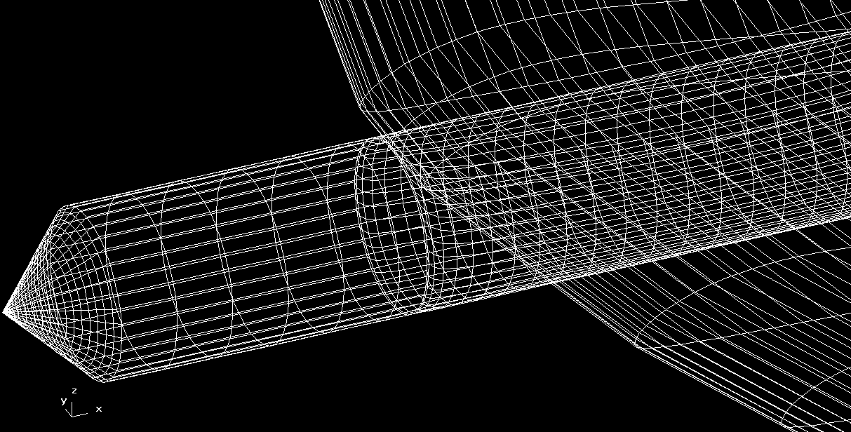
Cmarc by Aerologic is a tool for computational fluid dynamics.  The data generated by this program can be used to determine the flight properties of an aircraft, and with additional work can help determine the stability as well.  However, defining the geometry for the aircraft without the Aerlogic Loftsman tool is a difficult task.  This is due to the need to mesh various objects together when they intersect.  As with many things there are many ways to go wrong during this process and only one way to get it right.

Of particular interest is the connection between the aircraft’s body and the wing.  For the purposes of this project the case of wing attached to the top of a cylindrical body was explored.  The wing has no dihedral at the intersection and only the bottom of the wing touches the body.  The project was built to serve as an extension to Mavl with the code described below all being contained within a new class.

The geometry of the body is defined by two text files.  The first file contains the longitudinal profile (X-Z Plane) of the body as shown below.

The second file defines the lateral profile (Y-Z Plane) of the body.  The coordinates for this experiment were defined in polar coordinates to simplify the creation of the definition file.  Because the section is assumed to be mirrored, only 180 degrees of the profile is defined.  The result is the straight line shown below.

These last weeks have been quite a challenge with mounting school work and even a brief hospitalization (appendicitis).  Despite this my team and I have made great progress on our UAV.  The aircraft also has a name now “Vindication”.  We named the aircraft as such, because when completed. that it what the aircraft will become for all our hard work.

To address the challenge of creating a multi-configuration UAV I came up with the idea of using wing plate extensions.  However, in adding these extensions we did not want to have to readjust the center of gravity in order to maintain a static margin of 10%.  Thus the extensions are designed such that the change in neutral point due to the extensions is equal to the change in the center of gravity due to the added weight of the extensions.  This resulted in what we have been calling the “Lambda Wing” because of it’s transition from a swept wing to the straight wing.

Low Speed Configuration

There is still a long way to go.  The next step will be to model the aircraft in Cmarc which when properly completed will be considered our truth model.

High Speed Configuration

Both of these aircraft’s models were generated using the Mavl tool.  The tool’s functionality has grown considerably since its last mention hear, but it is interesting to note the the total line count has actually stayed almost constant at 1500 lines for the last eight weeks.  The rate at which code has been compressed has very coincidentally matched the rate at which new code is being added.  The Mavl tool is now fully capable of modelling an arbitrary aircraft (including control surfaces) as well as analyzing the stability and performance of the resultant aircraft.  The analysis tools include stall and cruise speed calculations thanks to the XFoil bridge being added.  It goes without saying that the tool is also capable of classifying the eigenvalues produced by AVL to determine the flight modes of the aircraft.  There is even a tool for correlating the flight modes to the handling levels as defined in MIL-F-8785.

Since I last wrote I have made significant progress on MAVL.  The program is now producing results like that shown below.  Full AVL model generation is now possible; rudders, elevators, and control surfaces are all possible now.  The capabilities of MAVL have been expanded to create and run test cases as well as load data from files created by AVL.

In particular, MAVL can read files created by the ST and SB commands under the OPER menu as well as reading the *.eig file created from the MODE menu.  This allows the user to create models from design parameters and get immediate stability information all with out leaving matlab.  The parseEig function also classifies the eigenvalues based on their relative orders of magnitude.  This allows the user to quickly access the phugoid, short period, dutch roll, spiral mode, and roll convergence.

Athena Vortex Lattice out of MIT is a great command line tool for analyzing the stability and control of an aircraft.  In developing the S&C for my senior design project I want to use AVL and Matlab together so for the past several hours I have been working on a matlab program that creates AVL models, tests them using AVL, and then loads the results data back into matlab.  The most basic version is now working (no control surfaces yet), but along the way there were some interesting bugs…