The Aerospace Design Toolbox is now available on Matlab Central.  This release includes examples on how to use the various functions to integrate with XFoil, AVL, and more.

I’ve recently switched to using Github for my open source projects.  As apart of this transition, I’ve been restructuring some of my old code.  This has lead to the creation of the aerospace-design-toolbox (ADT).

This Matlab toolbox is built from the Mavl code base.  The biggest difference between the two is scope.  While Mavl was designed to address the full scope of the design process from modeling to analysis, the ADT simply supports loading data from other aerospace software into Matlab.  Currently the ADT reads output files from AVL and Xfoil.  It can additionally read prop data in the format used by the UIUC propeller database.  For more information on what is and isn’t supported please see the README.m file in the repository.

At this time the toolbox is just a set of utility functions.  In the near term development will focus on converting the code into a standard toolbox that will integrate better with Matlab.

Mark Drela’s Athena Vortex Lattice (AVL)  program is a powerful tool for aerodynamic analysis.  Automating AVL runs using Matlab not only saves time, but eliminates human error when plugging through a large range of run cases.  In combination with tools for parsing the results and editing the models this automation may also enable design methods such as genetic algorithms and other iterative approaches.

Included below is a zip file containing the example script detailed here as well as a set of sample AVL files copied from the AVL source directory.  You will need to download AVL yourself and place the executable in the unzipped folder with the other files. Alternately, you may change the path to the avl executable in the last line of the script.  This tutorial was tested against avl 3.27.  Version 3.16 may have issues.

runAVL

Creating the run file

The run file to be created is simply a batch script that will be fed into AVL.  This will cause AVL to act as though the commands in the batch file are being typed in by a user.  The process begins by creating a blank file to put the batch script in.

%% Create run file %Open the file with write permission fid = fopen('.allegro.run', 'w');

Once this is complete, each line of the batch script is “printed” to the file by the fprintf command.  First, the aircraft’s avl and mass file are loaded into AVL.  The MSET command is executed to apply the mass parameters to all the run cases.  Then graphics are disabled to allow the program to run silently in the background.

%Load the AVL definition of the aircraft
fprintf(fid, 'LOAD %s\n', strcat(filename,'.avl'));

%Load mass parameters
fprintf(fid, 'MASS %s\n', strcat(filename,'.mass'));
fprintf(fid, 'MSET\n');
%Change this parameter to set which run cases to apply
fprintf(fid, '%i\n',   0); 

%Disable Graphics
fprintf(fid, 'PLOP\ng\n\n');

Once the setup is complete, the run case is defined and executed.  In this instance the C1 command is used to “set level or banked  horizontal flight constraints”.  The velocity is then set.  Depending on the purpose of the run case you may also use commands such as commented out under “Options for trimming”.  The case is then run using the X command.

%Open the OPER menu
fprintf(fid, '%s\n',   'OPER');   

%Define the run case
fprintf(fid, 'c1\n',   'c1');
fprintf(fid, 'v %6.4f\n',velocity);
fprintf(fid, '\n');

%Options for trimming %fprintf(fid, '%sn', 'd1 rm 0'); %Set surface 1 so rolling moment is 0 %fprintf(fid, '%sn', 'd2 pm 0'); %Set surface 2 so pitching moment is 0

%Run the Case
fprintf(fid, '%s\n',   'x');

Once the run is complete, the desired data in the OPER menu is saved to files for post analysis.  This example shows how to save the stability derivatives (ST) and body-axis derivatives (SB) data.  Other data that can be saved off in a similar fashion as shown below include:

• ST  stability derivatives
• SB  body-axis derivatives
• RE  reference quantities
• FT  total   forces
• FN  surface forces
• FS  strip   forces
• FE  element forces
• VM  strip shear,moment
• HM  hinge moments

%Save the st data
fprintf(fid, '%s\n',   'st');
fprintf(fid, '%s%s\n',basename,'.st');
%Save the sb data
fprintf(fid, '%s\n',   'sb');
fprintf(fid, '%s%s\n',basename,'.sb');

%Drop out of OPER menu
fprintf(fid, '%s\n',   '');

Other data may also be obtained by leaving the OPER menu and entering the MODE menu.  This eigenvalue data can be useful for analyzing an aircraft’s stability.

%Switch to MODE menu
fprintf(fid, '%s\n',   'MODE');
fprintf(fid, '%s\n',   'n');
%Save the eigenvalue data
fprintf(fid, '%s\n',   'w');
fprintf(fid, '%s%s\n', basename,'.eig');   %File to save to

%Exit MODE Menu
fprintf(fid, '\n');

Once all the desired runs have been computed and saved, it is important to use the return key character ‘n’ to return to the top level menu before issuing the Quit command to exit out of AVL and back to the command line. With the script complete the batch script file is closed.

%Quit Program
fprintf(fid, 'Quit\n'); 

%Close File
fclose(fid);

Executing the script

Files whose names conflict with new files to be generated should be moved out of the target directory or deleted before running the script.

[status,result] =dos(strcat('del ','allegro.st'));

Execution of the script from matlab is acheived by simply using the below command.  The dos command tells matlab to execute the string argument on the command line.  The instruction tells the OS feed the allegro.run file in the local directory to the avl executable at the absolute address shown.  The dos function also returns status and result data.  The status variable will get the final return state of the execution, nominally a 0 unless the program crashed.  The result variable will contain all the text that would have been printed to the screen if executed from the command line.

[status,result] = dos('C:avl.exe < .allegro.run');

With this complete the batch script will have successfully executed your run case or will have crashed.  To debug your batch script it is helpful to look through the result variable’s data.  Also helpful is to manually type in a script so that you can see more easily what the program is trying to do.

Solidworks is a great CAD program that can be useful in the design of aircraft.  However, one difficulty can be importing complex curves such as airfoils.  The challenge lies primarily in formatting the data such that solidworks can import it with its curves menu.  An example of properly formatted data is included below.

HS130

For data to be imported the file must contain X, Y, and Z coordinates in a tab-delimited file with no header.  Units may be included immediately after the number (“in” and “m” have been tested to work).  This can be accomplished with with an excel file by exporting the data as a tab-delimited file.  It may also be accomplished using the below python script to parse the data.  The script accepts arguements for filename (“-f” or “filename=”) and chord length in inches (“-c” or “chord=” ).  The airfoil data should be in a space-delimited file format.

foil2sldcrv

Once the data is ready to be loaded the process is fairly straight forward.

Solidworks Curves Menu

Clicking on the “Curve Through XZY Points” brings up a window from which the user may browse for a file containing their points.  This then allows the user to click “Browser” and select the file to import.

Curves menu with a sample airfoil loaded

Once this has been completed a “Curve” object is added to the Feature Manager, typically found on the left side of the screen.  The user may then create a sketch incorporating the airfoil data by using “Convert Entities” and then selecting the airfoil curve using the Feature Manager.  It is also advisable to right-click the curve on the Feature Manager and select “hide” so as to avoid future confusion.

Imported airfoil data with Feature Manager at right

Deleting the the “On Edge” constraints (the small green squares shown in the above image) will allow the airfoil to be moved and scaled as desired.  This may create a second airfoil to appear that is attached at the same ending point.  Simply deleting the second outline seems to be the easiest way to fix the problem.  Once the sketch is free to move you can then constrain it as needed.

Constrained Airfoil

Once the fuselage plug has been completed it may now be used as the basis for the fabrication of the fuselage molds.  This process starts with the fabrication of a parting plane.  The parting plane, as its name implies, is used to form the plane between the two halves of the fiberglass mold.  It will only be used for creating the first half of the mold.  The second half will be laid up against the first half.

To create the parting plane a rough cut slightly smaller than the body is made with a miter saw into a plywood piece.  This is then carefully sanded down so that the fuselage plug just fits.

Rough parting plane being sanded

Once the hole is finished, the entire board is sanded, painted, sanded again, and then waxed.  Once this is complete, the parting plane should have an almost mirror-like finish to it.

Mirror finish on completed parting plane

To support the parting plane and hold the plug halfway through the hole, a sub-structure is created under the parting plane.  It is important to ensure that holes drilled will be beyond the area over which fiberglass will be laid for the mold.

Parting plane with sub-structure and plug

Since the beginning of the semester we have made significant strides forward in building our senior design aircraft.  This post will focus on the fabrication of the fuselage plug.  The goal is to produce the fuselage geometry such that it may be used to create molds from which the actual aircraft skins may then be manufactured.

Render of the base plug to be created.

The core of the plug was made using a combination of foam and thin plywood.  As shown below, the plywood bulkhead serve to create the profile shape of the body while the lengthwise pieces of plywood serve to keep the bulkheads positioned and aligned correctly.  Foam blocks where then glued into the spaces and cut using a hot wire bow and a steady hand.  Once cut, the bulkheads are shimmed as needed and the gaps filled with epoxy.

Early stage of plug fabrication

To create the spherical nose of the aircraft, a foam ball from a crafts store was shaved down on a sanding belt until the correct circumference was had.  This was then epoxied to the front bulkhead.  Once all the foam was in place, the remaining seams and imperfections were covered in spackle and sanded down.

Plug covered in spackel ready for sanding

Next, the wing saddle is cut out of the plug.  This wing will sit such that the leading edge and trailing edge will sit flush with the body.  The cut is accomplished by clamping a plywood profile of the bottom of the wing to the plug.  Clamps, screws, and a plywood offset piece all work to keep the profile in place.  Again the cut is completed with a hot wire bow and a steady hand.

Plug ready for wing saddle to be cut

The last remaining feature to be added was the ventilation scope.  The basic shaped was cut out of foam using a template and the hot wire bow.  This was then glue to the plug.  A mix of Capasil and epoxy were then applied along the edge and smoothed with a gloved finger to create a bevel.  After curing, Bondo was used to create a smooth transition from the rear of the scoop to the body.

Initial scoop added to plug

With the plug shape complete, the plug was spackeled and sanded several times to get it as smooth as possible.  The plug was then fiberglassed and sanded.  The fiberglass plug was then touched up with Bono before once again being sanded and then spray painted.  A final wet sanding of the painted surface completed the construction of the plug.

Completed fuselage plug

For our senior design airplane we are building foam core wings.  The technique, which has been popular for years in the senior design program, involves cutting the wing shape out of foam which is subsequently encased in a composite shell.  To cut the wing shape we use a method called hot wire cutting.  As the name suggests, a heated wire is pulled along templates which melts the foam thus forming the wing.  During the process of cutting many wing shapes out of foam I have made some adjustments to the process in order to cut higher quality wings.  The process is particularly well suited to surfaces with blunt edges, but has not been tried on surfaces with taper where the technique may encounter challenges.

To cut the wings we require a number of tools and supplies:

1. Foam cut to the planform of the wing (We use highload 60 foam and leave at least a quarter of an inch extra at the leading and trailing edges)
2. Weights to hold the foam flat and stable
3. Wing profile shape (We cut ours using a laser cutter, we sure to sand the edges down as smooth as possible)
4. Bottom Edge profile with offset (Same requirements as the wing profile shape)
5. Screws and screwdriver
6. Hot wire bow
7. Power Supply (We use a BK Precision 1760 Desktop power supply)

A large clear workspace is desirable for this work.  The first step of the method is to place the profile and offset piece on the end of the wing.  The offset piece serves to position the airfoil a specific distance from the edge of the foam so that it is approximately centered in the foam.  The profile piece is then screwed in.  This is done on both ends of the foam.  We sure to notes which way the profile is facing when creating left panels versus right panels.

Now place the foam on the table where you will be cutting the piece and place plenty of weight on top.  This serves to prevent the piece from moving as well as keeping it flat on the surface.   The power supply is connected to the bow via clips which are connected close to the edge of the piece to be cut.

The power supply is set to “current mode” by using the leftmost switch located below the on/off switch.  The amount of amps that you will want to set your power supply to will vary based on the type of foam and the type of wire.  For cutting highload 60 and highload 40 insulation foam 1.58 amps +-0.1 amps proved to be the most effective.

The bow is now placed in front of and parallel to the leading edge of the piece.  The power supply is then turned on.  The bow string is pulled along the top edge of the offset piece and then over the top of the profile shape.  The wire outset the power clips will be cool allowing you to work the wire, but be careful to not touch the wire between the clips or the clips themselves.  During this process it is important to keep the bow taut against the profile and pull back at a slow steady pace (<1 cm/sec).  The bow string inside the piece will lag behind the string in your hands.  Try to limit this angle to less than 10 degrees.

Once you reach the end of the piece continue to pull the bow straight out the back.  Now remove the offset piece from the foam.  Placing the bowstring in front of the piece again pull the wire through the foam slightly above the first cut.  When you reach the profile shape pull the wire down and cut the underside of the profile using the same method as the top.

Once the bowstring reaches the end of the profile continue to pull it straight out the back of the foam.  Be sure to turn off the power supply.  You can now remove the weights and pull the foam beds away from the cut piece.

This method produced better results than other methods using the same profile pieces because the foam is always cutting against the wing profile shape.  This specifically prevents the wire from slipping or otherwise unintentionally cutting deeper into the foam than intended as long as the wire is kept at the proper angle across the block.

Also, because the wire is being pulled along the same profile for both the upper and lower cuts, what you see is what you get.  This is particularly evident on the trailing edge which came out perfectly straight and uniform during this example piece.

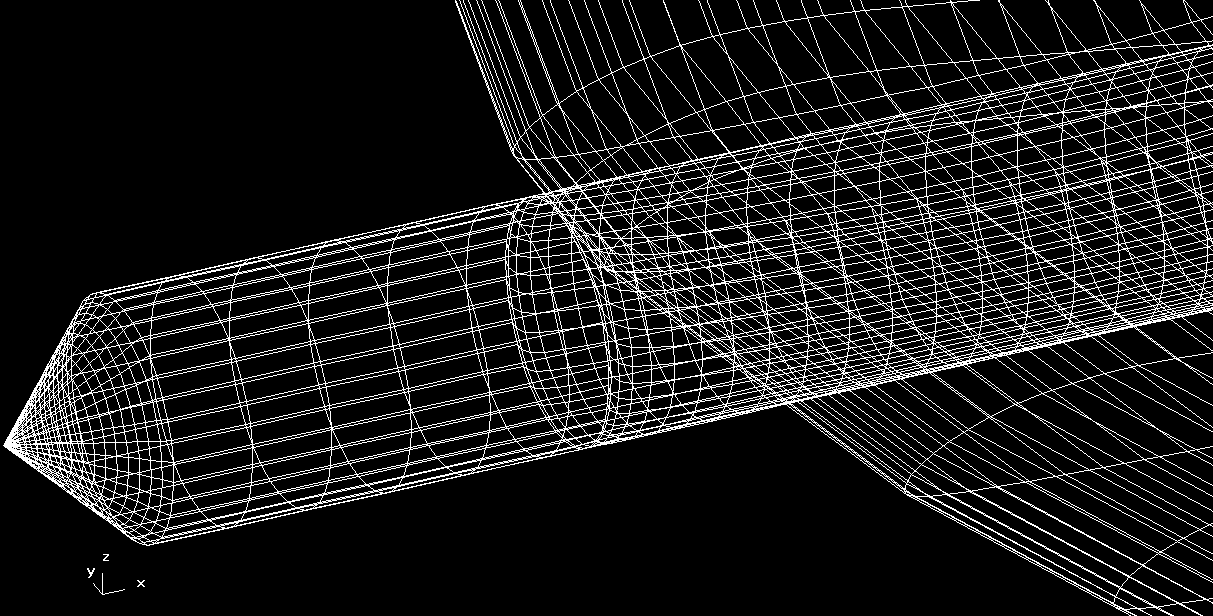
Cmarc by Aerologic is a tool for computational fluid dynamics.  The data generated by this program can be used to determine the flight properties of an aircraft, and with additional work can help determine the stability as well.  However, defining the geometry for the aircraft without the Aerlogic Loftsman tool is a difficult task.  This is due to the need to mesh various objects together when they intersect.  As with many things there are many ways to go wrong during this process and only one way to get it right.

Of particular interest is the connection between the aircraft’s body and the wing.  For the purposes of this project the case of wing attached to the top of a cylindrical body was explored.  The wing has no dihedral at the intersection and only the bottom of the wing touches the body.  The project was built to serve as an extension to Mavl with the code described below all being contained within a new class.

The geometry of the body is defined by two text files.  The first file contains the longitudinal profile (X-Z Plane) of the body as shown below.

The second file defines the lateral profile (Y-Z Plane) of the body.  The coordinates for this experiment were defined in polar coordinates to simplify the creation of the definition file.  Because the section is assumed to be mirrored, only 180 degrees of the profile is defined.  The result is the straight line shown below.

Since I last wrote I have made significant progress on MAVL.  The program is now producing results like that shown below.  Full AVL model generation is now possible; rudders, elevators, and control surfaces are all possible now.  The capabilities of MAVL have been expanded to create and run test cases as well as load data from files created by AVL.

In particular, MAVL can read files created by the ST and SB commands under the OPER menu as well as reading the *.eig file created from the MODE menu.  This allows the user to create models from design parameters and get immediate stability information all with out leaving matlab.  The parseEig function also classifies the eigenvalues based on their relative orders of magnitude.  This allows the user to quickly access the phugoid, short period, dutch roll, spiral mode, and roll convergence.

Athena Vortex Lattice out of MIT is a great command line tool for analyzing the stability and control of an aircraft.  In developing the S&C for my senior design project I want to use AVL and Matlab together so for the past several hours I have been working on a matlab program that creates AVL models, tests them using AVL, and then loads the results data back into matlab.  The most basic version is now working (no control surfaces yet), but along the way there were some interesting bugs…