Laser Cut Settings

Finding just the right settings for a laser cutter can be a time consuming guess and check process.  Additionally, using a calibration technique, such as the one detailed here, adds more time to the process of getting parts cut.  To ease this process here are the settings I use when cutting with a 60 watt Universal Laser Systems machine.

formica (add 0.003″ contour): Used to create smooth airfoil shapes.  The laser file does not store the z height settings.  You will need to turn on the z-axis and set a height of 0.025″.

WordPress Vulnerability

The recent outage of uavs.us was caused by a vulnerability in wordpress 2.8.4. Apparently, the “update” function in that version does not update wordpress beyond its current version. So despite making sure that it had downloaded the latest updates, the website remained stuck at version 2.8.4 for an extended period. More details on the exploit and repair work will be posted later.

Matlab AVL Control

%% Create run file
%Open the file with write permission
fid = fopen(strcat(basename,’.run’), ‘w’);
%Load the AVL definition of the aircraft
fprintf(fid, ‘LOAD %sn’, strcat(filename,’.avl’));
%Load mass parameters
fprintf(fid, ‘MASS %sn’, strcat(filename,’.mass’));
fprintf(fid, ‘MSETn’);
%Change this parameter to set which run cases to apply
fprintf(fid, ‘%in’,   0);
%Disable Graphics
fprintf(fid, ‘PLOPngnn’);
%Open the OPER menu
fprintf(fid, ‘%sn’,   ‘OPER’);
%Define the run case
fprintf(fid, ‘c1n’,   ‘c1’);
fprintf(fid, ‘v %6.4fn’,velocity);
fprintf(fid, ‘n’);
%Options for trimming
%fprintf(fid, ‘%sn’,   ‘d1 rm 0’);
%fprintf(fid, ‘%sn’,   ‘d2 pm 0’);
%Run the Case
fprintf(fid, ‘%sn’,   ‘x’);
%Save the st data
fprintf(fid, ‘%sn’,   ‘st’);
fprintf(fid, ‘%s%sn’,basename,’.st’);
%Save the sb data
fprintf(fid, ‘%sn’,   ‘sb’);
fprintf(fid, ‘%s%sn’,basename,’.sb’);
%Drop out of OPER menu
fprintf(fid, ‘%sn’,   ”);
%Switch to MODE menu
fprintf(fid, ‘%sn’,   ‘MODE’);
fprintf(fid, ‘%sn’,   ‘n’);
%Save the eigenvalue data
fprintf(fid, ‘%sn’,   ‘w’);
fprintf(fid, ‘%s%sn’, basename,’.eig’);   %File to save to
%Exit MODE Menu
fprintf(fid, ‘n’);
%Quit Program
fprintf(fid, ‘Quitn’);
%Close File
fclose(fid);

Mark Drela’s Athena Vortex Lattice (AVL)  program is a powerful tool for aerodynamic analysis.  Automating AVL runs using Matlab not only saves time, but eliminates human error when plugging through a large range of run cases.  In combination with tools for parsing the results and editing the models this automation may also enable design methods such as genetic algorithms and other iterative approaches.

Included below is a zip file containing the example script detailed here as well as a set of sample AVL files copied from the AVL source directory.  You will need to download AVL yourself and place the executable in the unzipped folder with the other files. Alternately, you may change the path to the avl executable in the last line of the script.  This tutorial was tested against avl 3.27.  Version 3.16 may have issues.

runAVL

Creating the run file

The run file to be created is simply a batch script that will be fed into AVL.  This will cause AVL to act as though the commands in the batch file are being typed in by a user.  The process begins by creating a blank file to put the batch script in.

%% Create run file %Open the file with write permission fid = fopen('.allegro.run', 'w');

Once this is complete, each line of the batch script is “printed” to the file by the fprintf command.  First, the aircraft’s avl and mass file are loaded into AVL.  The MSET command is executed to apply the mass parameters to all the run cases.  Then graphics are disabled to allow the program to run silently in the background.

%Load the AVL definition of the aircraft
fprintf(fid, 'LOAD %s\n', strcat(filename,'.avl'));

%Load mass parameters
fprintf(fid, 'MASS %s\n', strcat(filename,'.mass'));
fprintf(fid, 'MSET\n');
%Change this parameter to set which run cases to apply
fprintf(fid, '%i\n',   0); 

%Disable Graphics
fprintf(fid, 'PLOP\ng\n\n');

Once the setup is complete, the run case is defined and executed.  In this instance the C1 command is used to “set level or banked  horizontal flight constraints”.  The velocity is then set.  Depending on the purpose of the run case you may also use commands such as commented out under “Options for trimming”.  The case is then run using the X command.

%Open the OPER menu
fprintf(fid, '%s\n',   'OPER');   

%Define the run case
fprintf(fid, 'c1\n',   'c1');
fprintf(fid, 'v %6.4f\n',velocity);
fprintf(fid, '\n');

%Options for trimming %fprintf(fid, '%sn', 'd1 rm 0'); %Set surface 1 so rolling moment is 0 %fprintf(fid, '%sn', 'd2 pm 0'); %Set surface 2 so pitching moment is 0

%Run the Case
fprintf(fid, '%s\n',   'x');

Once the run is complete, the desired data in the OPER menu is saved to files for post analysis.  This example shows how to save the stability derivatives (ST) and body-axis derivatives (SB) data.  Other data that can be saved off in a similar fashion as shown below include:

  • ST  stability derivatives
  • SB  body-axis derivatives
  • RE  reference quantities
  • FT  total   forces
  • FN  surface forces
  • FS  strip   forces
  • FE  element forces
  • VM  strip shear,moment
  • HM  hinge moments
%Save the st data
fprintf(fid, '%s\n',   'st');
fprintf(fid, '%s%s\n',basename,'.st');
%Save the sb data
fprintf(fid, '%s\n',   'sb');
fprintf(fid, '%s%s\n',basename,'.sb');
%Drop out of OPER menu
fprintf(fid, '%s\n',   '');

Other data may also be obtained by leaving the OPER menu and entering the MODE menu.  This eigenvalue data can be useful for analyzing an aircraft’s stability.

%Switch to MODE menu
fprintf(fid, '%s\n',   'MODE');
fprintf(fid, '%s\n',   'n');
%Save the eigenvalue data
fprintf(fid, '%s\n',   'w');
fprintf(fid, '%s%s\n', basename,'.eig');   %File to save to

%Exit MODE Menu
fprintf(fid, '\n');

Once all the desired runs have been computed and saved, it is important to use the return key character ‘n’ to return to the top level menu before issuing the Quit command to exit out of AVL and back to the command line. With the script complete the batch script file is closed.

%Quit Program
fprintf(fid, 'Quit\n'); 

%Close File
fclose(fid);

Executing the script

Files whose names conflict with new files to be generated should be moved out of the target directory or deleted before running the script.

[status,result] =dos(strcat('del ','allegro.st'));

Execution of the script from matlab is acheived by simply using the below command.  The dos command tells matlab to execute the string argument on the command line.  The instruction tells the OS feed the allegro.run file in the local directory to the avl executable at the absolute address shown.  The dos function also returns status and result data.  The status variable will get the final return state of the execution, nominally a 0 unless the program crashed.  The result variable will contain all the text that would have been printed to the screen if executed from the command line.

[status,result] = dos('C:avl.exe < .allegro.run');

With this complete the batch script will have successfully executed your run case or will have crashed.  To debug your batch script it is helpful to look through the result variable’s data.  Also helpful is to manually type in a script so that you can see more easily what the program is trying to do.
Rapid Prototyping Nose Cones

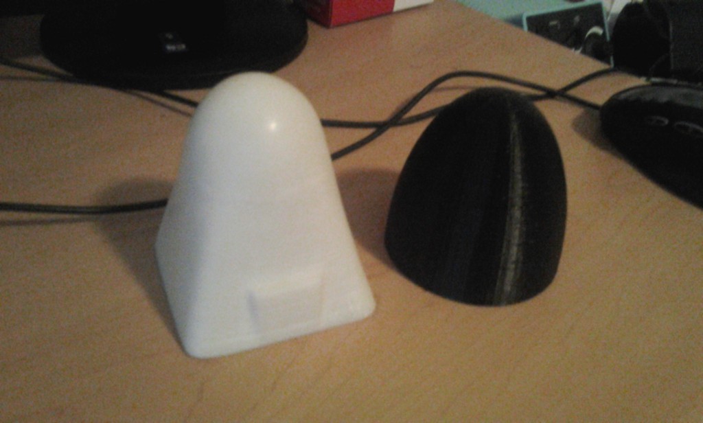
One of the compelling reasons for buying a Reprap Mondo was the potential for printing aircraft molds and parts.   Keeping with this goal, the Reprap Mondo was used to print the nose cone shown below in white ABS.  Its basic geometry is based on my senior design aircraft’s nose.  Recently I obtained access to an Ultimaker via the Entrepreneurship Initiative’s Garage.  Using the Ultimaker an elliptical nose cone was printed in black PLA.

Printed Nose Cones

Printed Nose Cones

The white nose cone pictured has been sanded and polished while the black cone is raw off the printer.  Overall the surface finish was similar between the two pieces.  Both did suffer from surface defects including an instance on both prints when their respective printers stopped extruding for a moment causing a large defect.  The white ABS cone did have the advantage that most of its defects were positive allowing them to be sanded while the black PLA cone has regular pit defects.  This is attributed to the ultimaker switching from the outer shell to the inner surface at such high speed.

Since the quality of the finished parts is rather close, the biggest difference between them is the time it took to print.  While the Mondo spent 6 hours printing the ABS piece, the Ultimaker only took 1.5 hours.  The comparison is not the best since the objects are distinctly different, but the conclusion stands that the Ultimaker is much much faster than the Mondo.

The difference in the materials is not particularly apparent in the final products.  Both parts are rigid, easy to sand, and fairly indestructible.  Since the parts are intended for use as molds, the strength to weight consideration is not present as it would be in flyable parts.  The important difference during this experiment was the ease of printing.  To prevent the ABS cone from warping it needed a heated bed, a heat gun, and super glue to ensure that it stayed on the platform.  The PLA cone needed none of this and printed just fine.

The one advantage that the Mondo has over the Ultimaker is its larger print volume.  However, the difficulties of printing in ABS have precluding actually using that greater volume.  Based on this, further work shall focus on the use of PLA as the material of choice.

RepRap Mondo – Part 8 – Belts

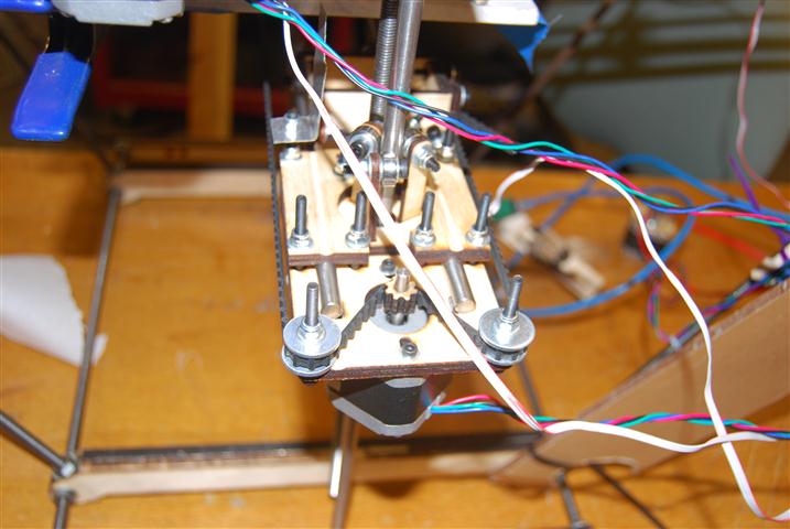
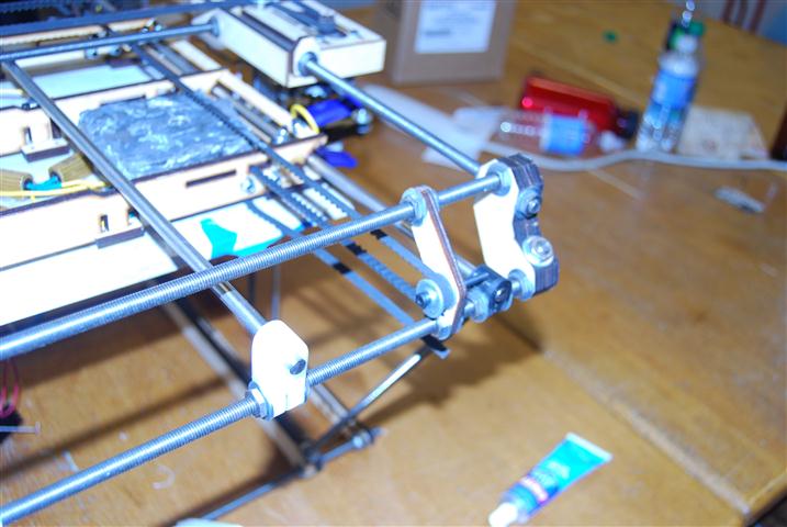
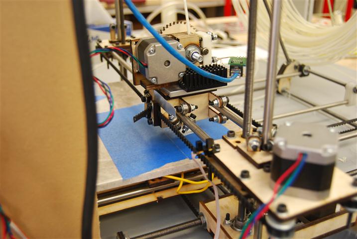
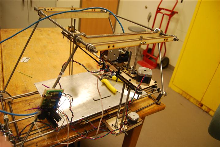
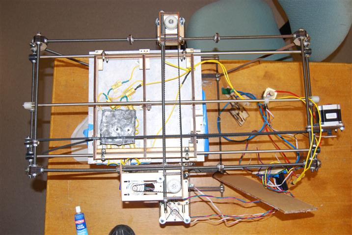
The RepRap Mondo has three belts that need to be installed.  An overview of the belts as seen from the bottom of the machine is shown below.  The large lead block under the bed is just pinning down the resistors while the adhesive cures and is not apart of the machine.

Bottom view of the machine

Bottom view of the machine

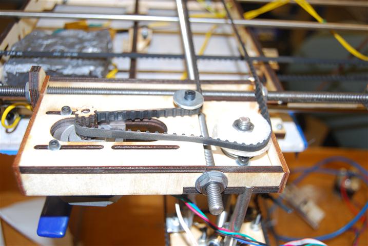
The belt slips over the idlers and motors previously installed on the Y-Axis.  The belt ends are then clamped to the head mount under light tension.

Elevator Belts

Elevator Belts

The Z-axis belt is a continuous loop and is installed under light tension.  The belts should not rub against any other structures.  The idler wheel shown below is built similarly to those on the elevator.

Z-axis belts

Z-axis belts

The X-axis idler simply mounts to the opposite end of the machine to the X-axis motor.  The ends of the belt are clamped to the bottom of the bed.

X-axis idler

X-axis idler

RepRap Mondo – Part 7 – Endstops

The RepRap Mondo’s mechanics are one of its strongest attributes, however in designing the machine it appears that the endstops were completely forgotten.  As a result of this and a complete lack of instructions, the locations and mounts for all the endstops shown are based only on our conjecture, but having run our machine for a while now we can confirm that these positions do work.

The cables that came with the endstops do not fit properly on the pins from the endstop.  As a result, they have a tendency to pop off.  We cut off the ends an soldered them directly to the contacts inside the end-stops.  These were exposed by cutting part of the end-stop enclosure off.

X end-stop

X end-stop

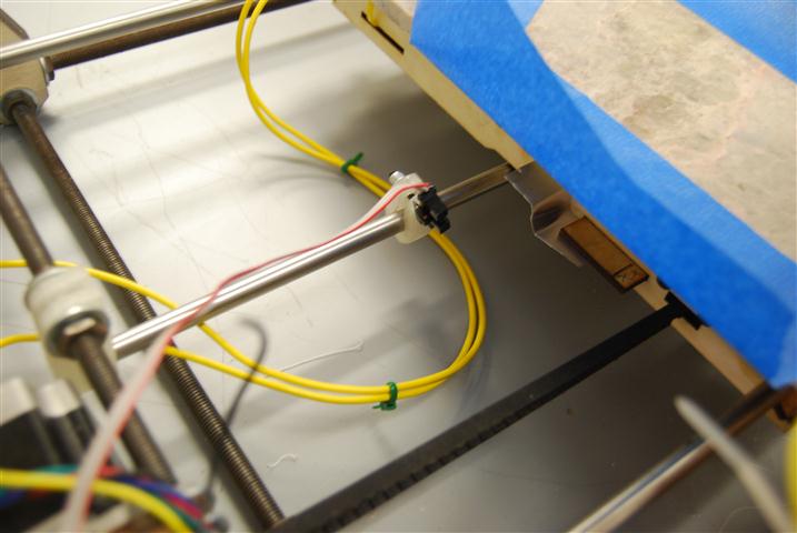
The X-axis end-stop sensor was mounted to an extra hole we conveniently found on the elevator assembly.  The kit ships with a piece of thin aluminum that we cut down to the size shown.  The belt clamp was loosened and the aluminum plate was slipped in.  On tightened down the clamp held the aluminum quite well.  There is a small angle cut into the bottom of the aluminum plate so that if it gets bumped down the angle will cause the piece to get pushed back up instead of being mangled.

Y End-stop

Y End-stop

The Y end-stop sensor mounts to a small RepRapped piece which slides over the Y axis smooth rods.  A bolt clamps the rod and holds the sensor.  A small piece of wood was glued to the bed to make a small shelf to mount the aluminum piece.  The Z-bend in the aluminum makes it easier to adjust.  The aluminum is super-glued to the bed frame shelf.  To clear the deck, the sensor is bent back at a slight angle.   It would probably also work to mount the sensor rotated 180 to avoid needing to tilt it.

The Y end-stop sensor is mounted so far forward in the above picture because our marble bed is currently 6 inches shorter than the warped 18″ bed that the kit shipped with.

Z End-stop

Z End-stop

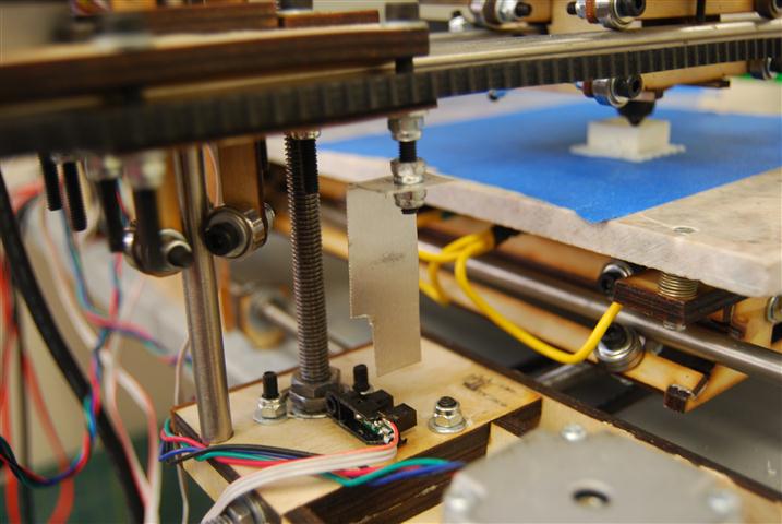
To mount the Z End-stop we glued the sensor on its side to the base of the elevator.  We then cut a hole in the aluminum piece and used lock-nuts to attach it to the bottom of one of the screws used int he elevator assembly.  This is the only end-stop mount that is finely adjustable and is so specifically because you will need to tune this axis the most.  Slight adjustments can make a big difference.

RepRap Mondo – Part 6 – The Bed

Aluminum Bed

The Mondo ships from Techzone with an aluminum bed.  The 18″ x 12″ bed comes with six holes for mounting to the base support.  Although the holes are nicely chamfered they did not include machine screws to go with the holes.  None of the screws that fit through the holes were flush with the bed either.  After hitting one of the bolt heads with the extruder nozzle we made a run to the hardware store to get a pack of 4-40 1″ screws with nuts.
Techzonecom warped metal bed

Techzonecom warped metal bed

With the proper screws in place we then set about leveling the bed.  Several hours later I discovered that the bed was badly warped such that no amount of tweaking would make it flat.  We measured a tip deflection of 3-4 mm near the ends which was a significant problem given that the layer thickness was 0.4 mm.  For a while we continued printing by restricting the build area to a three inch square near a corner we leveled relative to the head.

Glass Bed

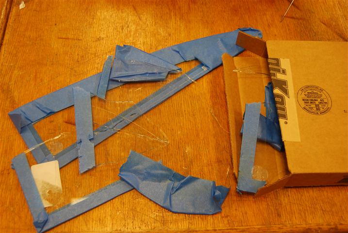
This deficiency in the bed lead us to our first alternate bed made from 3mm glass, which turned out to be 2.3 mm when meaured with calipers.  The 18″ x 12″ glass bed was cut for us and only cost $5.  It was mounted on top of the aluminum bed by placing six blobs of “clear silicone, waterproof sealant” that we picked up from the hardware store.  We selected it based on its tolerance of heat up to 175 degrees Celsius which was above any of the temperatures we expected the bed to see.  Once the glass was set on the silicone we then shimmed and squished down the bed as needed to get it level.
Remains of the glass bed

Remains of the glass bed

However, during later prints we found that heating the bed with a heat gun resulted in superior print quality with reduced warping.  Unlike the metal bed which nicely conducted the heat through out, the glass bed required that heat be applied locally at the printing area.  Although this arrangement worked for a while, as we tried to increase the local temperature the local heating eventually caused a crack to form across the bed starting from a chip on the edge.  The glass bed wasn’t destroyed at that point, but rather as we tried to get the glass bed off we had to resort to breaking the bed down into more manageable, albeit razor sharp, sections.

Marble Bed

It was at this point that the suggestion was made that we try a thin ceramic material used as a base material in thick film circuit deposition.  It was quickly determined that there was no local supplier and the material would be expensive.  However, 3/8″ granite and marble floor tiles are cheaply available at the local hardware store and come in 12″ and 18″ squares.  For this first experiment we purchased a 12″ marble tile for $2.28.
Marble bed installed

Marble bed installed

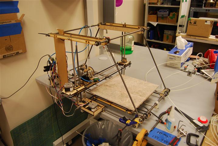
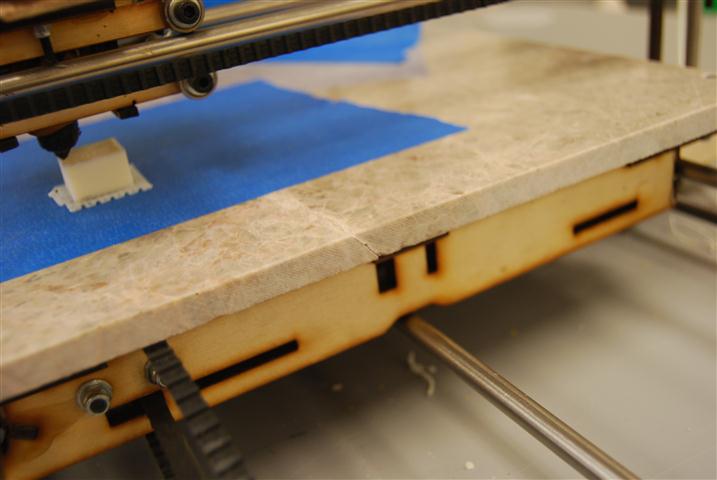
The marble bed has proven over the last week to be incredibly flat, durable, and gorgeous.  Mounting to the bed support was accomplished by drilling four holes with a tile bit set before then chamfering the holes with a larger bit.  It is also noteworthy that although this bed takes a while to heat up, once it is hot it tends to stay hot for an extended period of time.
The only problem he have had is in our selection of an individual tile. The tile that we selected had a natural crack running through it that was visible on both the top and bottom of the tile.  The crack is more obvious when the bed is heated up.  Despite this, once a printing surface is laid down, such as the painter’s tape shown, the crack has no effect on the usability of the surface.
A natural crack in the marble

A natural crack in the marble

RepRap Mondo – Part 5 – Stepper Motor

The RepRap Mondo requires 4 motors for the three axes of motion and the extruder.  Three of these motors have four wires, but the Y-axis motor is larger and has six wires.  Techzonecom cut the white and yellow wires short presumably so that the person using this motor would not make the mistake of using them.  However, as we soon demonstrated, there is no color coding associated with stepper motors.

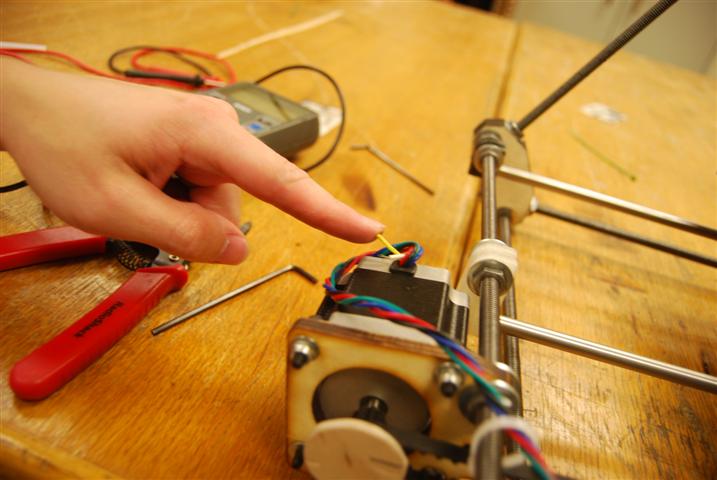
When we wired up the Y-axis motor using the same color pattern as the smaller motors we observed very unusual behavior.  The bed moved smoothly in the positive direction, but when commanded to go in the negative direction the bed shook violently and continued to move in the positive direction.  Using an Ohm meter Michael Yenik, my partner on this project, determined that the blue wire was in fact a center tap on the motor instead of being the end of the coil.  After soldering an extension on to the yellow wire, which was connected to the end of the coil, and connecting it in place of the blue wire we were able to get the bed to smoothly move in both directions.

Stepper motor with needed wire cut short

Stepper motor with needed wire cut short

Importing Airfoils into Solidworks

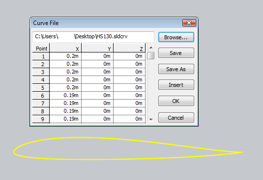
Solidworks is a great CAD program that can be useful in the design of aircraft.  However, one difficulty can be importing complex curves such as airfoils.  The challenge lies primarily in formatting the data such that solidworks can import it with its curves menu.  An example of properly formatted data is included below.

HS130

For data to be imported the file must contain X, Y, and Z coordinates in a tab-delimited file with no header.  Units may be included immediately after the number (“in” and “m” have been tested to work).  This can be accomplished with with an excel file by exporting the data as a tab-delimited file.  It may also be accomplished using the below python script to parse the data.  The script accepts arguements for filename (“-f” or “filename=”) and chord length in inches (“-c” or “chord=” ).  The airfoil data should be in a space-delimited file format.

foil2sldcrv

Once the data is ready to be loaded the process is fairly straight forward.

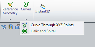
Solidworks Curves Menu

Solidworks Curves Menu

Clicking on the “Curve Through XZY Points” brings up a window from which the user may browse for a file containing their points.  This then allows the user to click “Browser” and select the file to import.

Curves menu with a sample airfoil loaded

Curves menu with a sample airfoil loaded

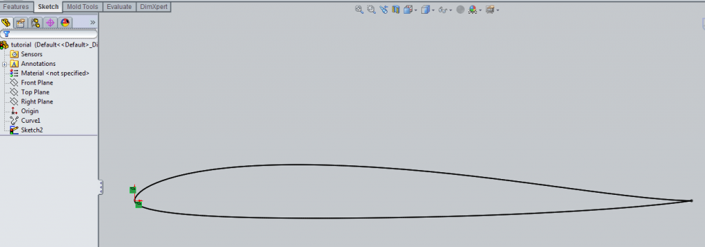
Once this has been completed a “Curve” object is added to the Feature Manager, typically found on the left side of the screen.  The user may then create a sketch incorporating the airfoil data by using “Convert Entities” and then selecting the airfoil curve using the Feature Manager.  It is also advisable to right-click the curve on the Feature Manager and select “hide” so as to avoid future confusion.

Imported airfoil data with Feature Manager at right

Imported airfoil data with Feature Manager at right

Deleting the the “On Edge” constraints (the small green squares shown in the above image) will allow the airfoil to be moved and scaled as desired.  This may create a second airfoil to appear that is attached at the same ending point.  Simply deleting the second outline seems to be the easiest way to fix the problem.  Once the sketch is free to move you can then constrain it as needed.

Constrained Airfoil

Constrained Airfoil

RepRap Mondo – Part 4 – Extruder

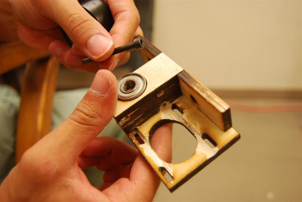
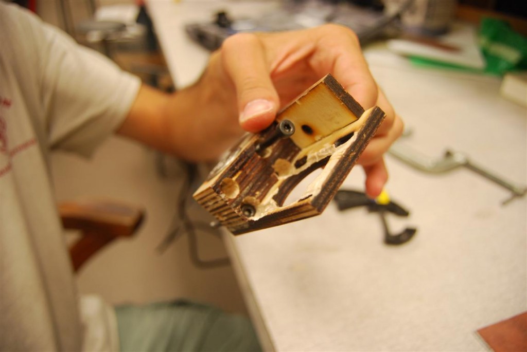
The extruder seemed like it would be an easy component to assemble thanks to good instructions on the reprap site.  However, it quickly became evident that techzone’s laser cut version was going to be a much greater challenge.   The first issue that arose was that the screws closest to the motor mount could not be inserted into the holes until we routed the channels as shown in the below image.

Wade's Extruder with minor alterations

Wade's Extruder with minor alterations

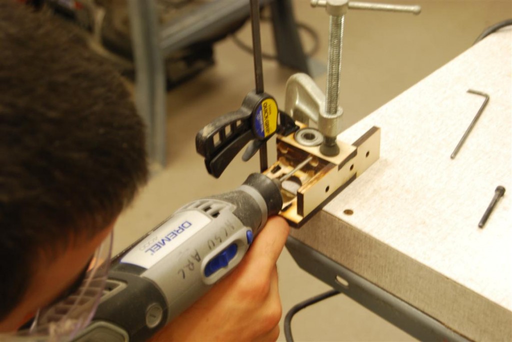
Further modifications were required because the screw heads could did not clear the motor.  To fix this, extra material was routed out to make room for them.  The challenge of this is quite evident below.

Modifications in progress

Modifications in progress

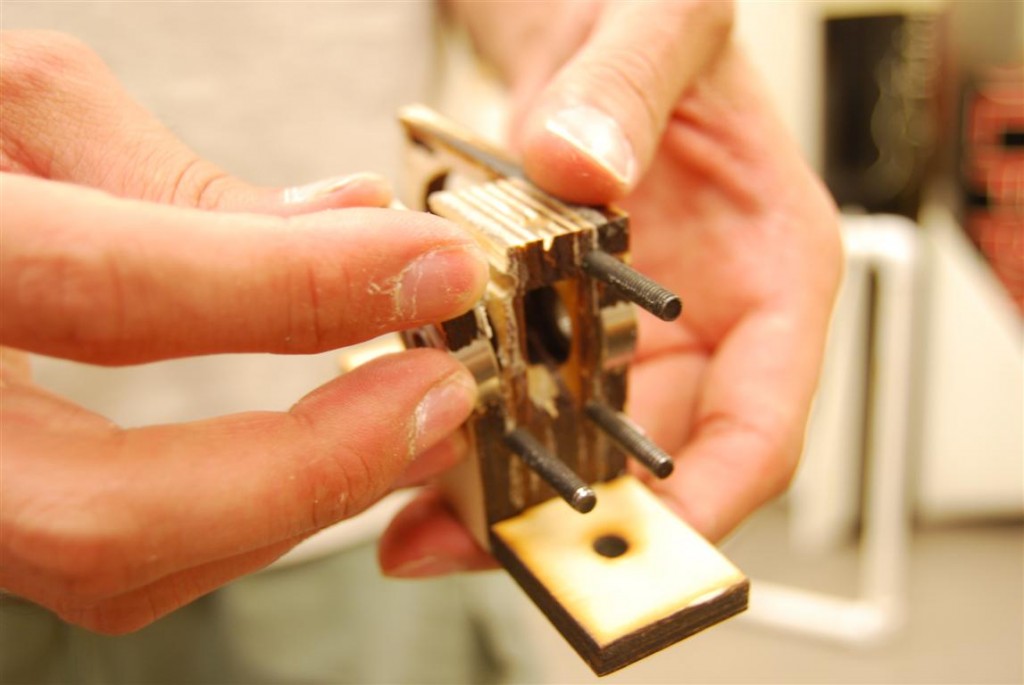
These holes would also need to be made deeper to allow the screws to stick out far enough for springs and nuts to be added on the other side.

Modifications complete

Modifications complete

Bolts sticking out the appropriate distance

Bolts sticking out the appropriate distance

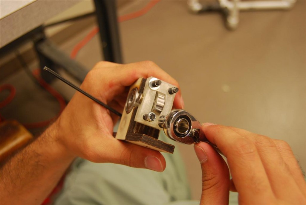
After much modification, we were finally able to get the assembly put together.  Between the two top pictures you can see that the screw holes for mounting the extruder to the reprap are covered by the motor and spring assembly making it impossible to swap the extruder without a complete disassembly of the device.

Assembly of the feeder

Assembly of the feeder

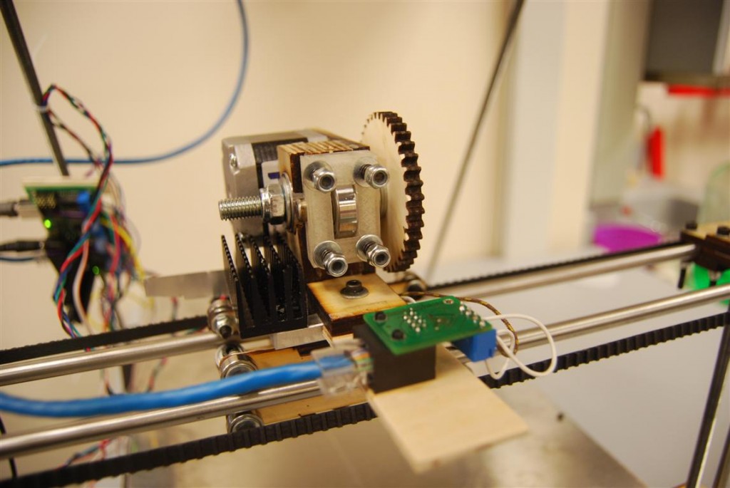
The motor, gears, and extruder drive shaft were then assembled.  One thing we learned later during tuning is that washers need to be added to the extruder drive shaft such that the gripping surface is aligned with the filament.

Extruder finished and mounted

Extruder finished and mounted

The tuning process was mostly concerned with the tension of the four springs.  The problem was that the springs can only be adjusted with the motor removed.  This necessitated the removal of the drive shaft as well because the large gear blocks access to the motor’s mounting screws.

Return top